In addition to the on-the-fly 2D denoising integrated in the UI, Warp includes a command line tool that allows to train a denoising neural network on volumetric data using the noise2noise principle. You will find Noise2Map.exe inside the installation directory. Add this directory to your PATH environment variable so you can execute the tool more comfortably in the respective data folder. Launch the tool without any parameters to print a list of the available options.

Noise2Map will likely require two GPUs to be present in your system, or a single one with a lot of memory (16+ GB).

3D denoising can work on two types of data: Half-map reconstructions from single particle data, and tomograms.

Denoising half-maps

When applied to half-maps, the denoising will produce a map filtered to local resolution. Noise2Map can operate on one or multiple pairs of half-maps. While we haven’t observed any additional benefits from training a model on multiple pairs, you may be more lucky, especially if all maps have similar amounts of noise.

The first map of each pair must be put in one folder (e. g. “odd”), and the second into another folder (e. g. “even”). The file names must be identical between the two folders, otherwise Noise2Map can’t match them. Specify the two folders in the –observation1 and –observation2 arguments.

One common binary mask can be provided to assist the tool in balancing the number of protein and solvent training samples, and to improve the amplitude spectrum flattening. Inside the mask, voxels corresponding to protein must have the value 1. No soft edge is needed. Specify the mask path in –mask.

The amplitude spectrum can be flattened beyond the 1/10Å spatial frequency to provide a similar effect to B-factor-based sharpening. This is enabled by default and can be disabled by setting –dont_flatten_spectrum. You can tune the flattening by changing –overflatten_factor. The Fourier components will be multiplied by (1 / rotational_average)^overflatten_factor, i. e. the default value of 1 results in normal flattening, a value of 0 disables the flattening, and a value above 1 leads to additional sharpening. The flattening requires the –angpix parameter to be set to reflect the pixel size in Å. Please note that the denoising process will still dampen the initially flat amplitudes if they are considered too noisy, possibly resulting in a visually less “sharp” map than traditional B-factor sharpening.

If the global resolution of the maps is far below the Nyquist frequency, setting –lowpass (in Å) to a somewhat higher value (and specifying –angpix) can improve the results in some cases. Please note that setting this parameter to the global resolution value will make you miss out on the possibly higher local resolution in some parts of the map. On the other hand, if the resolution is close to Nyquist, you might want to use the –upsample parameter with a value bigger than 1 to upscale the maps prior to denoising.

The default number of 600 training –iterations usually produces good results for SPA-derived half-maps. To save GPU memory, you can set –batchsize to less than 4, and the number of iterations will be adjusted accordingly. If you have a GPU with a lot of memory, you can try a batch size bigger than 4.

Once the training is finished, Noise2Map will combine the half-maps and denoise their average. You can force it to denoise each half-map separately by specifying –denoise_separately. This can be interesting when using the denoised half-maps in 3D refinement.

The denoised maps will be saved in the denoised folder.

If you’ve already trained a model and would like to apply it to similar data or with different output settings (e. g. –denoise_separately = true), you can specify the model name as –old_model. Noise2Map will save the trained model as noisenet3d_64_xxxxxx in the current directory. Please note that changing filtering parameters such as –flatten_spectrum, –lowpass etc. will likely invalidate models trained with different settings.

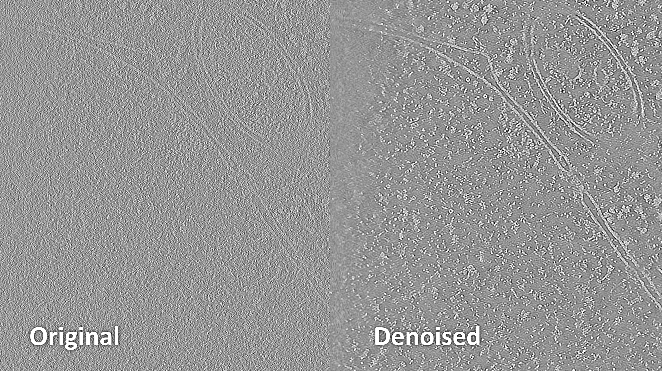
Denoising tomograms

Data preparation for tomogram denoising isn’t as straight-forward as with SPA-derived half-maps. We’ve obtained the best results by using pairs of tomograms reconstructed from all odd, and all even tilt images, respectively. You can now easily create such training data in Warp by ticking the “Separate odd/even tilts for denoising” checkbox in the full tomogram reconstruction dialog – the volumes will be saved to “odd” and “even” subfolders. If you also tick “Also produce deconvolved version”, the training data will be pre-deconvolved, resulting in a look more similar to what Warp produces for 2D data. If the tomograms contain only a small region of interest, you might want to crop them to that area to avoid training on mostly empty areas.

The rest of the workflow is very similar to the half-map section above, so we will only point out the differences here:

–dont_flatten_spectrum should be set.
–mask should not be specified.
–iterations must be set to a much higher value in our experience, above 10 000. However, you might want to try lower values for your data first.

Tomogram denoising will likely suffer from a small pixel size, as it adds unnecessary noise at spatial frequencies known not to contain any interpretable information in a single reconstruction, e. g. beyond 20 Å.